Stencils for Fun and Profit

Written by Julian Samaroo

Of all the foundational HPC algorithm varieties, stencils are probably the most fun. In simulations, stencils implement cool physics-based effects like fluid dynamics, heat transfer, and chemical reactions. In image and video processing, they power blur, edge detection, and sharpening. In machine learning, they form the computational core of every convolutional neural network. And if you're a Dagger user, all of these are within arm's reach — with full parallelism across CPU threads, distributed workers, and GPUs — using a single expressive macro.

TL;DR

• @stencil is a macro for expressing element-wise operations on DArrays that can also access neighboring elements, and it parallelizes itself across your hardware resources automatically.

• @neighbors(A[idx], distance, BC) returns the neighborhood of A around idx as a flat array, with a boundary condition of your choice applied.

• Supported boundary conditions include Wrap, Pad, Clamp, Reflect (symmetric and mirror), and LinearExtrapolate, and can be mixed per dimension.

• @stencil runs the same code on CPU threads, distributed workers, and GPUs based on Dagger's configured scope — no code changes needed to switch between them.

• Current limitation: all DArrays in a single @stencil call must share the same size, shape, and chunk partitioning. This will be relaxed in future versions.

---

What's a Stencil?

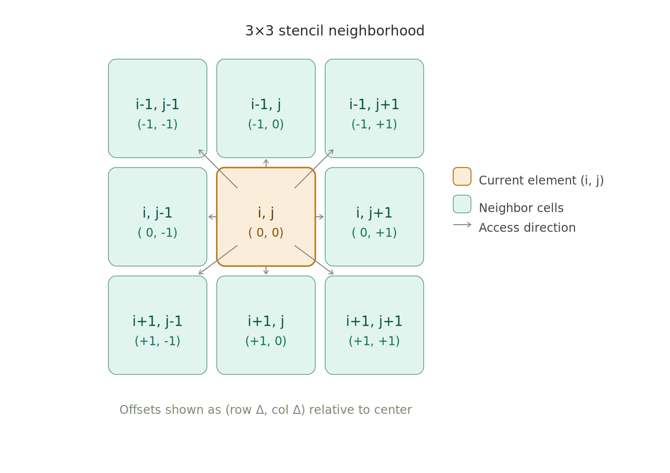
A stencil is an element-wise operation over a grid of values, where the output at a given point can depend not just on the current value but on neighboring values too.

Think about simulating how a chemical diffuses across a 2D grid. To find the new concentration at point (i, j), you need to know the concentrations at (i-1, j), (i+1, j), (i, j-1), and (i, j+1) — because diffusion is driven by concentration gradients, meaning the chemical moves from high-concentration regions to low-concentration ones. That pattern of reaching out to the surrounding neighborhood is exactly what makes stencils different from a plain map.

The neighborhood size can be 1 (a 3x3 grid in 2D), 2 (5x5), or even non-uniform per dimension — more on that later.

---

The Mental Model

At its core, @stencil works like a parallel for loop over every element of your DArray(s). Inside the loop, idx is the current element's index, and @neighbors(A[idx], distance, BC) gives you the neighborhood values around that index as a flat array.

import Dagger: @stencil, Wrap

A = ones(Blocks(2, 2), Float64, 8, 8)
B = zeros(Blocks(2, 2), Float64, 8, 8)

@stencil B[idx] = sum(@neighbors(A[idx], 1, Wrap())) / 9.0

Here, B[idx] gets the average of the 3×3 neighborhood of A centered at idx. The 1 is the neighborhood radius, and Wrap() means that accesses outside the array bounds wrap around to the opposite side — like a torus.

A few important things to keep in mind:

• @stencil primarily reads and writes DArray objects. If you pass a plain Array (like a convolution kernel), it's treated as a global constant shared across all elements — useful for kernels and coefficients.

• All DArrays used inside a single @stencil expression must have the same size, shape, and chunk partitioning. This will be relaxed in future versions.

The multi-expression form of @stencil lets you chain operations within a single parallel pass:

uvv = similar(u)
@stencil begin
    uvv[idx] = u[idx] * v[idx]^2
    u[idx] += Du * (sum(@neighbors(u[idx], 1, Wrap())) / 9.0 - u[idx]) - uvv[idx]
end

And if you don't have an output array constructed yet, @stencil can allocate one for you:

B = @stencil sum(@neighbors(A[idx], 1, Wrap()))
# B is a new DArray with the same shape and partitioning as A

---

Diffusion

Let's start with the classic diffusion example and build it up properly. We want to simulate how a chemical spreads across a 2D grid over time, starting from a small source at the center.

using Dagger
import Dagger: @stencil, Wrap
using Statistics

C = zeros(Blocks(10, 10), Float64, 100, 100)
@view(C[50:51, 50:51]) .= 1.0

We've created a 100×100 distributed array, partitioned into 10×10 chunks, with a small source of chemical at the center. Now for the stencil:

function diffuse!(C; rate=0.1)
    @stencil C[idx] += rate * (mean(@neighbors(C[idx], 1, Wrap())) - C[idx])
end

This is the discrete diffusion equation: the new concentration at each point is the old concentration, adjusted toward the local average. mean(@neighbors(C[idx], 1, Wrap())) gives the average of the 3×3 neighborhood (the 8 surrounding cells and C[idx] itself).

After one step, the chemical barely moves. After 100 steps, it has spread significantly:

for _ in 1:100
    diffuse!(C)
end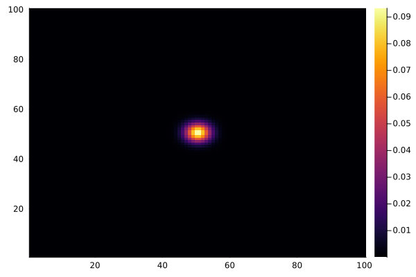

And to animate the process:

using Plots

C .= 0.0
@view(C[50:51, 50:51]) .= 1.0

anim = @animate for _ in 1:100
    diffuse!(C)
    heatmap(collect(C), clim=(0, 1))
end
gif(anim, "diffusion.gif", fps=15)

---

Reaction-Diffusion: Gray-Scott

Diffusion alone gets boring. Let's try something wilder: the Gray-Scott model, a classic reaction-diffusion system where two chemicals u and v interact in a way that produces striking organic-looking patterns.

The model is governed by:

∂u/∂t = Du·∇²u - u·v² + f·(1 - u)
∂v/∂t = Dv·∇²v + u·v² - (f + k)·v

The Laplacian term ∇²u is approximated by the difference between u at a point and its local neighborhood average — the same structure as diffusion. The u·v² term is the reaction: u is consumed by v, and v feeds on u.

using Dagger
import Dagger: @stencil, Wrap

u = ones(Blocks(100, 100), Float64, 200, 200)
v = rand(Blocks(100, 100), Float64, 200, 200) .* 0.3

# Seed the center
@view(u[95:105, 95:105]) .= 0.5
@view(v[95:105, 95:105]) .= 0.25

function gray_scott!(u, v; f=0.055, k=0.062, Du=0.16, Dv=0.08)
    lap_u = similar(u)
    lap_v = similar(v)
    uvv = similar(u)
    @stencil begin
        lap_u[idx] = mean(@neighbors(u[idx], 1, Wrap())) - u[idx]
        lap_v[idx] = mean(@neighbors(v[idx], 1, Wrap())) - v[idx]
        uvv[idx] = u[idx] * v[idx]^2
        u[idx] += Du * lap_u[idx] - uvv[idx] + f * (1 - u[idx])
        v[idx] += Dv * lap_v[idx] + uvv[idx] - (f + k) * v[idx]
    end
end

The @stencil begin...end block processes all expressions together, so intermediate values like uvv are computed in-order with u and v. Note that lap_u, lap_v, and uvv are DArrays with the same partitioning as u and v — they have to be, since @stencil requires all DArray operands to share the same structure. This is why we need to use similar to create them (which preserves the partitioning).

After a few thousand iterations with the "coral" parameter set (f=0.055, k=0.062), the patterns emerge:

anim = @animate for i in 1:200
    gray_scott!(u, v; f=0.055, k=0.062)
    heatmap(collect(v), c=:inferno, colorbar=false)
end
gif(anim, "gray-scott.gif", fps=20)

Different parameter sets produce entirely different behaviors — coral, spots, stripes, spirals. The Gray-Scott model has been extensively mapped, and the ready.io parameter explorer is a great place to experiment.

---

Image Convolution

Convolutions are the stencil you're most likely familiar with if you've worked in computer vision or machine learning. A convolution takes a small fixed-size array (the "kernel") and for each element of the input, computes a weighted sum of the neighborhood values, where the weights come from the kernel.

This is exactly what @stencil is built for. The kernel is a plain Array — since it's not a DArray, it's treated as a global constant and broadcast to all workers automatically.

using Dagger, Images
import Dagger: @stencil, Pad

# Load image as an RGB/RGBA DArray
img_raw = load("input-image.jpg")
image = DArray(img_raw, Blocks(64, 64))
output = similar(image)

# 15x15 box blur kernel
kernel = fill(1/225, 15, 15)

@stencil output[idx] = clamp01(sum(@neighbors(image[idx], 7, Pad(0.0)) .* kernel))

Here, Pad(0.0) fills out-of-bounds accesses with zeros, which is the standard choice for image convolutions — it prevents edge artifacts from wrapping or clamping.

The .* kernel broadcast multiplies the neighborhood element-wise with the kernel before summing. Because kernel is a plain Array, @stencil passes it through as-is — it's not indexed with idx.

The input image:

after being blurred with a 15x15 box blur kernel above becomes:

The same pattern works for other kernels:

import Dagger: Clamp

# Sobel edge detection (horizontal component)
sobel_x = [
    -1  0  1;
    -2  0  2;
    -1  0  1
]
edges = @stencil clamp01(sum(@neighbors(image[idx], 1, Pad(0.0)) .* sobel_x))

# Sharpening
sharpen = [
     0  -1   0;
    -1   5  -1;
     0  -1   0
]
sharp = @stencil clamp01(sum(@neighbors(image[idx], 1, Clamp()) .* sharpen))

Sobel edge detection:

Sharpening:

---

Heat Diffusion with Insulating Boundaries

The Wrap() boundary condition we used for diffusion treats the grid as if it wraps around — physically, this models a periodic domain, like a simulation on a torus. But most real physical domains have actual edges. A common physical boundary condition is the insulating (Neumann) boundary: no heat (or chemical, or field) flows through the wall. In the discrete setting, this is equivalent to reflecting the grid values at the boundary, so the gradient at the edge is zero.

That's exactly what Reflect(true) does. Symmetric reflection means that the value just outside the boundary is treated as equal to the value just inside — making the finite-difference gradient at the edge zero and preventing any net flux through the wall.

Let's set up a 2D heat diffusion problem with a hot rod along one edge and insulating walls everywhere:

using Dagger, Plots
import Dagger: @stencil, Reflect

T = zeros(Blocks(20, 20), Float64, 100, 100)

# Hot rod along the bottom edge
@view(T[end, :]) .= 1.0

The stencil is the same finite-difference Laplacian as before, just with a different boundary condition:

function diffuse_insulating!(T; rate=0.3)
    @stencil T[idx] += rate * (mean(@neighbors(T[idx], 1, Reflect(true))) - T[idx])
end

After 500 iterations:

anim = @animate for _ in 1:500
    diffuse_insulating!(T)
    heatmap(collect(T), c=:hot, title="Insulating walls, hot base")
end
gif(anim, "$(@__DIR__)/heat-reflect.gif", fps=20)

Compare this with the same setup using Wrap(): heat from the bottom edge would bleed out the top and reappear at the bottom, which is unphysical for a bounded domain. With Reflect(true), the walls are genuinely insulating — heat accumulates and distributes, but none escapes.

The Reflect(false) (mirror) variant is slightly different: it skips the boundary element itself during reflection, which enforces a stricter zero-gradient condition and is sometimes preferred in spectral methods. For most physical diffusion problems, Reflect(true) is the natural choice.

---

Boundary Conditions

As we've seen, one of the places @stencil really shines is its range of boundary conditions. When a neighborhood access goes outside the array, something has to fill in the missing value. The right choice depends on your problem:

Wrap() — out-of-bounds accesses wrap around to the opposite side, as if the array is a torus. Good for periodic simulations.

import Dagger: Wrap

@stencil B[idx] = sum(@neighbors(A[idx], 1, Wrap()))
# 4|1234|1

Pad(value) — out-of-bounds accesses return a constant fill value. Zero padding is standard for image convolutions and finite-domain PDEs.

import Dagger: Pad

@stencil B[idx] = sum(@neighbors(A[idx], 1, Pad(0.0)))
# 0|1234|0

Clamp() — out-of-bounds accesses are clamped to the nearest boundary element. Good when you want boundary values to "hold" rather than wrap or pad.

import Dagger: Clamp

@stencil B[idx] = sum(@neighbors(A[idx], 1, Clamp()))
# 1|1234|4

Reflect(true) (symmetric) and Reflect(false) (mirror) — out-of-bounds accesses are reflected back into the array. Symmetric reflection repeats the edge element; mirror reflection does not. Both are common in signal processing.

import Dagger: Reflect

@stencil B[idx] = sum(@neighbors(A[idx], 1, Reflect(true)))   # symmetric
# 1|1234|4
@stencil B[idx] = sum(@neighbors(A[idx], 1, Reflect(false)))  # mirror
# 2|1234|3

LinearExtrapolate() — extends the boundary by extrapolating the slope at the edge. Useful when you expect the field to continue smoothly beyond the domain. Only supports Real element types.

import Dagger: LinearExtrapolate

@stencil B[idx] = sum(@neighbors(A[idx], 1, LinearExtrapolate()))
# 0.0|1.0 2.0 3.0|4.0

You can also mix boundary conditions per dimension by passing a tuple. For example, a simulation that wraps in the x-direction but pads in the y-direction:

import Dagger: Wrap, Pad

@stencil B[idx] = sum(@neighbors(A[idx], 1, (Wrap(), Pad(0.0))))

---

Multi-Dimensional Stencils and Non-Uniform Neighborhoods

@stencil works in any number of dimensions — 1D, 2D, 3D, and beyond. The neighborhood distance can be specified as a scalar (same in all dimensions) or as a tuple (different per dimension).

# 1D stencil with distance 2 (neighborhood of 5 elements)
A = DArray([1.0, 2.0, 3.0, 4.0, 5.0, 6.0], Blocks(3))
B = similar(A)
@stencil B[idx] = sum(@neighbors(A[idx], (2,), Wrap()))

# 3D stencil with asymmetric neighborhood
# distance (1, 2, 1) → 3×5×3 neighborhood
A3 = rand(Blocks(4, 5, 3), Float64, 8, 10, 6)
B3 = similar(A3)
@stencil B3[idx] = mean(@neighbors(A3[idx], (1, 2, 1), Wrap()))

For the chunk size requirement: each chunk dimension must be at least as large as the neighborhood distance. If your chunk is too small for the neighborhood distance, you'll get an error.

---

GPU Support

Moving a stencil to the GPU requires exactly zero changes to the stencil code itself. You control execution via Dagger's scope system — within a GPU scope, allocate your DArrays and call your @stencil, and it will be compiled for and run on the GPU.

using Dagger, CUDA
import Dagger: @stencil, Wrap

gpu_scope = Dagger.scope(cuda_gpu=1) # Use the first CUDA GPU

Dagger.with_options(; scope=gpu_scope) do
    C = zeros(Blocks(32, 32), Float32, 512, 512)
    @view(C[255:256, 255:256]) .= 1.0f0

    for _ in 1:200
        @stencil C[idx] += 0.1f0 * (mean(@neighbors(C[idx], 1, Wrap())) - C[idx])
    end
end

The same works for AMD (ROCm), Intel oneAPI, Apple Metal, and OpenCL — just load the appropriate backend and use the corresponding scope key (rocm_gpu, intel_gpu, metal_gpu, cl_device). For multi-GPU setups, use cuda_gpus=: to spread DArray chunks across devices.

---

Other Applications

Stencils are a surprisingly general pattern. Beyond diffusion and convolutions, @stencil can support:

Cellular automata — Conway's Game of Life, for example, is a stencil where the next state of each cell is determined by the count of live neighbors. Rule-based cellular automata like Wolfram's elementary automata are 1D stencils.

PDE solvers — finite difference methods for wave equations, the heat equation, Poisson's equation, and many others are all stencil operations. The Jacobi and Gauss-Seidel iterative solvers for linear systems have stencil structure too.

Morphological operations — binary erosion and dilation (used in image segmentation and shape analysis) are stencils over boolean arrays. Grayscale morphology generalizes this to min/max neighborhood operations.

Smoothed-particle hydrodynamics (SPH) — density estimation kernels in SPH are computed over neighborhoods, fitting naturally into the stencil model.

Finite element method assembly — element stiffness contributions from neighboring nodes can be expressed as stencils on structured grids.

---

Putting It Together

A few practical points before you go:

The @stencil macro handles all the chunk boundary communication for you — when a neighborhood access crosses a chunk boundary, Dagger knows to fetch the needed halo values from the neighboring chunk's location, whether that's another thread, another process, or another GPU. You never see this machinery; you just write the neighborhood expression.

Performance-wise, @stencil is most effective when your array chunks are large enough to amortize the halo communication overhead. As a rule of thumb, chunk sizes in the hundreds-per-side range tend to work well in practice; tiny chunks push the overhead-to-work ratio in the wrong direction.

Not everything you need is implemented yet, but we're very open to feature requests!

---

References

• Dagger.jl documentation: Stencil Operations

• Dagger.jl repository: github.com/JuliaParallel/Dagger.jl

• Gray-Scott parameter explorer: mrob.com/pub/comp/xmorphia

CC BY-SA 4.0 Julian P. Samaroo. Last modified: March 12, 2026.